Manipulation of base modification data

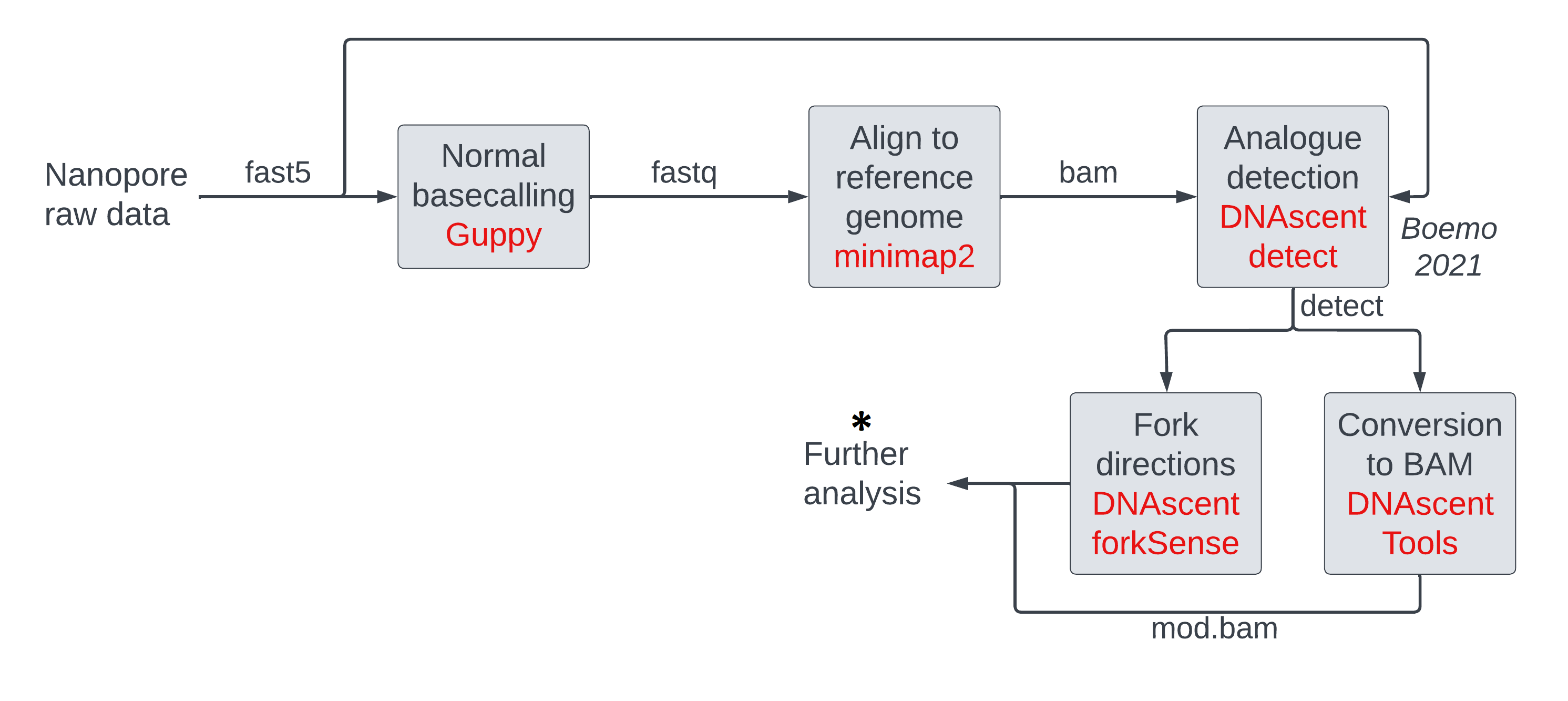
In this session, we will look at commands that manipulate modification data in mod BAM and produce summary statistics or plots. Some of these commands are similar to those run behind the scenes in a visualization software. By running these commands ourselves, we get quantitative output in a tabular format instead of an image format, and we can manipulate this data further in our own scripts/pipelines. These steps are all in the ‘further analysis’ section of our pipeline and must be tuned or tailored to the experiment at hand by the experimenter.

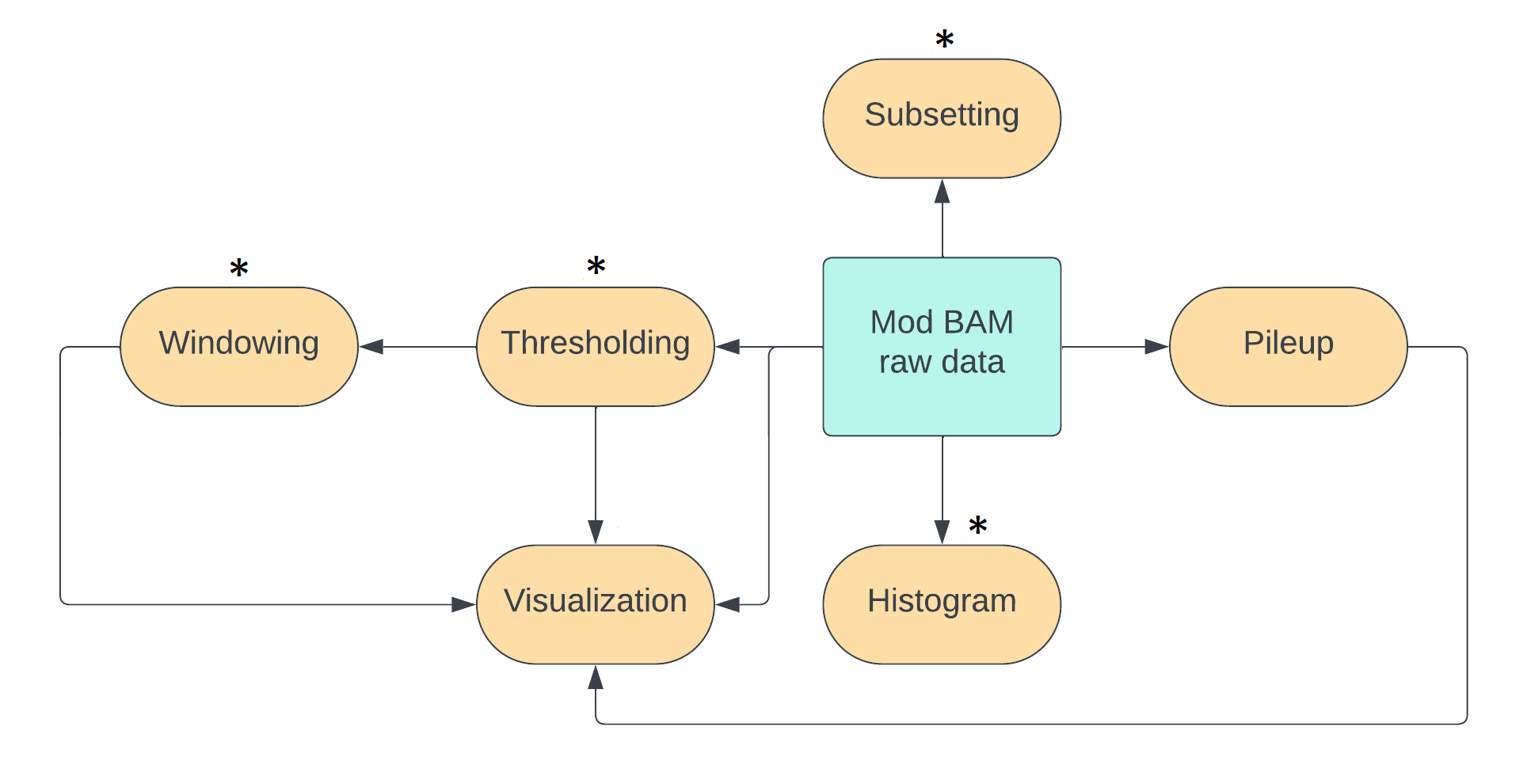
The operations we will be running on mod BAM files are:

• thresholding
• making histograms of modification probabilities
• subsetting (either randomly, or by genomic location, or by mean modification density)
• windowing modification calls

We can achieve most of these operations using the pre-existing packages modkit and samtools. For windowing and for measuring mean modification densities across reads, we will use our own tools due to an absence of ready-made tools. In a later session, we will use the package modbamtools for further manipulation.

Simple thresholding of mod BAM files with modkit

Thresholding is the process of converting soft modification calls to hard calls i.e transforming a probability of modification per base per sequenced strand to a binary yes/no. The ground truth for an experimental sample is that every base on a DNA strand is either modified or unmodified. The probability of modification associated with every base in a mod BAM file is due to uncertainty in the measurement procedure and this accumulates from different stages of our experiment and subsequent analysis, all the way from sample preparation to modification calling on a computer. For some applications, we just want a simple yes/no answer to the modification question and this uncertainty is not important.

There are two ways of thresholding, and they can be applied separately or together:

• thresholding directly on modification probabilities,
• thresholding on model confidences.

We will be using just thresholding directly on probabilities, and leave thresholding on model confidences to optional sections below.

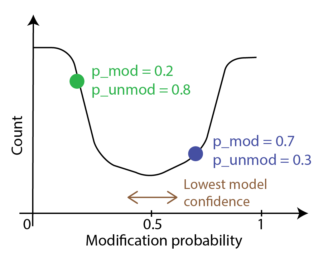
The probability curve of modification per base usually looks like the following image. Each point on the curve corresponds to a probability of modification p_mod and a probability that the base is unmodified p_unmod; these add up to 1. The calls with probabilities close to zero or one are where the model in the modification caller is certain that the call is correct. The calls around 0.5 are where model uncertainty is the highest as it is doing no better than an unbiased coin toss.

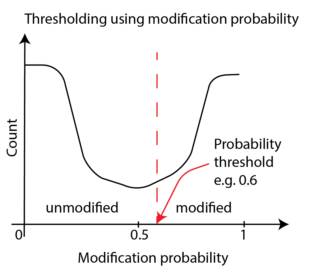
To threshold directly on probabilities, we convert bases with the probability of modification p_mod above a threshold value into modified and bases with p_mod below that value into unmodified. The simplest threshold value is 0.5. If one wanted to make an informed choice about a threshold, one has to generate the histogram, examine it, and make a decision - we will cover this later in this session.

We can execute the thresholding step with a threshold of 0.5 using modkit.

input_mod_bam= # fill suitably
output_mod_bam= # fill suitably
modkit call-mods --no-filtering $input_mod_bam $output_mod_bam

Run modkit extract on the input and output mod bam files. You will see that the modification probability is now either a value very close to zero or a value very close to one.

(optional) Multiple modifications

Please note that if there are multiple modifications, a base can exist in more than two states: unmodified, modification of the first type, modification of the second type etc. Now call-mods assigned the state with the highest measured probability to the base.

Syntax for thresholds other than 50%

If we want to use a threshold other than 0.5, the syntax is

input_mod_bam= # fill suitably
output_mod_bam= # fill suitably
mod_code= # fill with mod code. e.g.: T for our BrdU data, m for 5mC.
threshold= # fill with a number between 0 and 1.
modkit call-mods --mod-threshold $mod_code:$threshold \
  --filter-percentile 0 $input_mod_bam $output_mod_bam

(optional) Using model confidences as thresholds

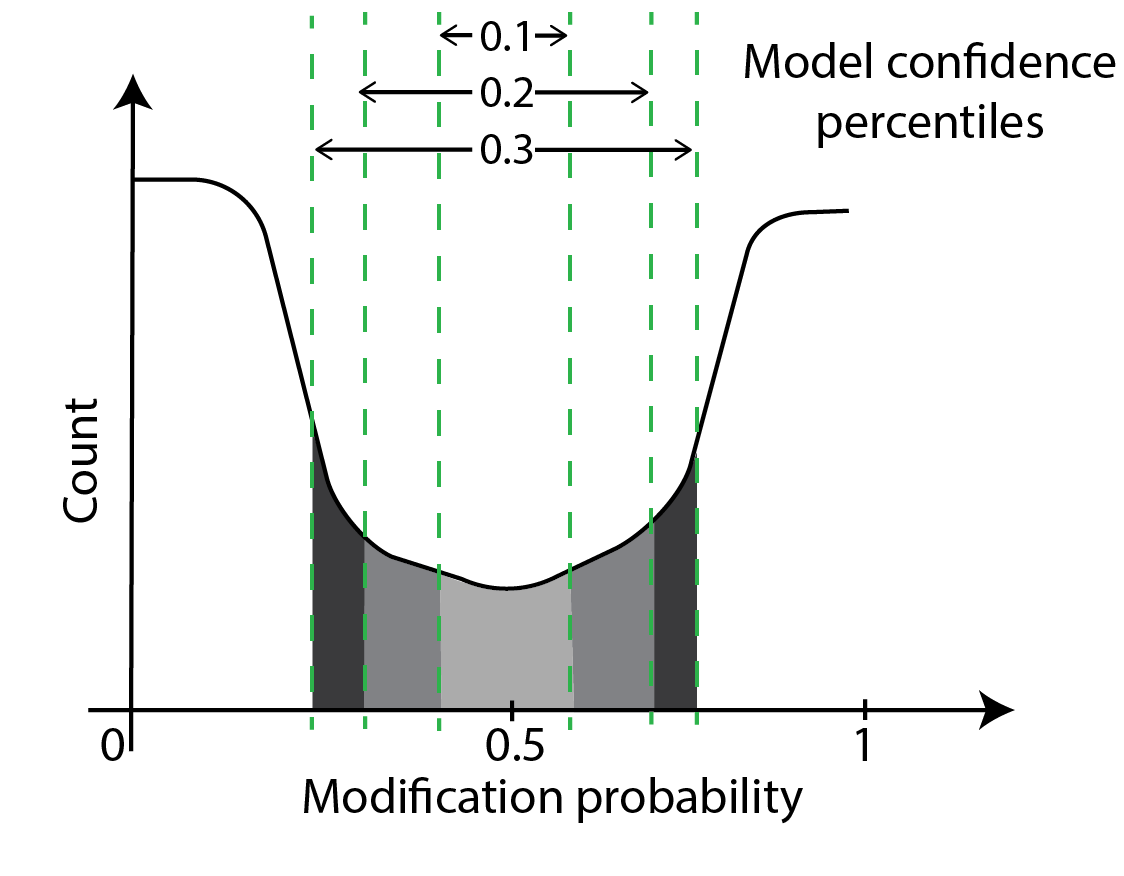
Another way to perform thresholding is through model confidences. Model confidence is highest at bases with modification probabilities close to zero or one. At these bases, the model is very confident that the base is unmodified or modified respectively. Model confidence is lowest at bases with modification probabilities close to 0.5. Here, the model is saying it can do no better than an unbiased coin toss. A schematic of confidence percentiles on a modification-probability curve is shown below. As you can see, model confidences grow as one moves away from the midpoint of 0.5 in either direction. Model confidence is not a new measurement - we are just asking which parts of the probability curve around the center have areas a fraction of the whole curve with the fraction set at 10%, 20% etc.

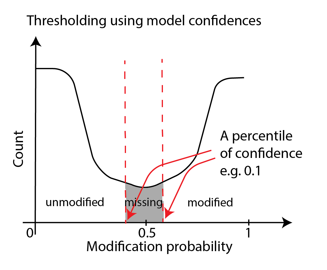
One can threshold using the percentiles of confidence as shown below. In principle, we are moving high-confidence model calls to the modified or unmodified category and discarding the low-confidence model calls. This approach is similar to the simple thresholding we have discussed thus far but we use two thresholds here and the probabilities corresponding to the two thresholds is not known beforehand.

This thresholding is accomplished through the --filter-percentile and/or the --filter-threshold options of modkit call-mods, which may be used standalone or in addition to the --mod-threshold parameter. We will not be discussing this further; you can refer to the modkit documentation here if you are interested.

Histograms of modification probabilities using modkit

In this section, we will calculate histograms of per-base modification probabilities. One of its uses is helping us choose a threshold for a thresholding step that we were discussing above. Another use is to see if our experiment worked and we are seeing an expected number of bases with modifications.

We will use the modkit sample-probs command. We operate the tool in the histogram mode --hist and want ten bins in the histogram (--buckets 10), and wish to sample 1000 reads (-n 1000) to measure statistics (we are using 1000 to save runtime; usually a fraction of the BAM file is sufficient for these calculations and we leave it to the experimenter to determine what that fraction is for their dataset). We will discuss the -p option in an optional subsection a little later.

NOTE: The modkit sample-probs command produces tabular files with rows labeled with either an unmodified one-letter code or a modified one-letter code. In the case of 5mC methylation which is coded as C+m, the rows are labelled either C or m. In the case of a generic modification such as T+T, which we use to label our BrdU data, we run into problems because both the modified and the unmodified rows are labeled T. This is a problem with the modkit sample-probs tool. To get around the problem, before using this tool, we change the T+T code to T+B using modkit adjust-mods. This is not a good idea in general as B means not A in the standard one-letter nucleotide code list. But, as the modification field is still developing, we occasionally run into these problems and have to use such workarounds.

input_mod_bam= # fill this suitably
input_mod_bam_adjust_tag= # fill this suitably

# convert mod BAM from using T+T to T+B
modkit adjust-mods --convert T B $input_mod_bam \
  $input_mod_bam_adjust_tag
samtools index $input_mod_bam_adjust_tag

# sample probabilities and make a histogram
cd ~/nanomod_course_outputs/yeast
modkit sample-probs -p 0.1,0.2,0.3,0.4,0.5 \
  $input_mod_bam_adjust_tag -o ./histogram --hist --buckets 10 -n 1000

The output files are deposited in the ./histogram folder. You should see three output files: probabilities.txt, probabilities.tsv and thresholds.tsv. The probabilities files report number of modified bases in ten buckets of modification probability p_mod from 0.5 - 1.0, and the same for the number of unmodified bases using the probability that the base is not modified p_unmod = 1 - p_mod. probabilities.txt also contains a histogram made with ASCII art (i.e. using the symbol ∎ to build horizontal bars of this histogram).

Have a look at these files, and answer this question for yourself: what would be a good modification probability value for thresholding?

(optional) thresholds.tsv: measure correspondence between model confidence thresholds and direct probability thresholds

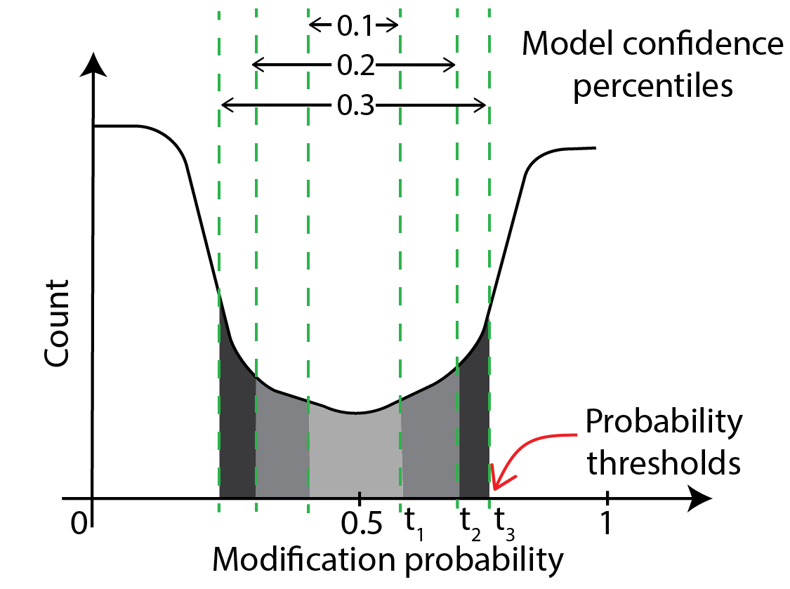
thresholds.tsv contains the table of conversion between model confidences and direct probability thresholds. This is illustrated in the schematic below, which shows that model confidences of 10% and below lie between modification probabilities of t_1 and 0.5 - t_1, confidences of 20% and below lie between t_2 and 0.5-t_2 etc. So, thresholds.tsv contains a table that lists this correspondence. There are a few other details such as how the program deals with probability curves that are not symmetric about 0.5. We are not going to discuss this further; please experiment with this tool and read the documentation to learn more.

Form modification histogram from data only at given genomic regions

To form a histogram from data restricted to given genomic regions, pass a BED file containing these regions to modkit sample-probs with the --include-bed option. In the command block below, we look for modification probabilities in the regions chrI:100000-200000 and chrVII:500000-600000. In other words, the program calculates statistics from bases on reads that fall in either region.

input_mod_bam= # fill this suitably
input_mod_bam_adjust_tag= # fill this suitably
regions_bed_file= # we are going to make this file

# convert mod BAM from using T+T to T+B
modkit adjust-mods --convert T B $input_mod_bam \
  $input_mod_bam_adjust_tag

# one can use any regions and any number of regions in the commands
# below. The '.' in the sixth column means we include both +
# and - strands in our calculation.
echo -e "chrI\t100000\t200000\tA\t1000\t." > $regions_bed_file;   
echo -e "chrVII\t500000\t600000\tB\t1000\t." >> $regions_bed_file;

# sample probabilities and make a histogram
cd ~/nanomod_course_outputs/yeast
modkit sample-probs -p 0.1,0.2,0.3,0.4,0.5 \
  $input_mod_bam_adjust_tag -o ./histogram_subset --hist --buckets 10 -n 1000 \
  --include-bed $regions_bed_file

(optional) Use modkit motif-bed to form bed files for motifs

To form a BED file for particular motifs such as CG, you can use the modkit motif-bed command. Please refer to the modkit documentation for more details.

Subsetting mod BAM files with samtools

We take a mod BAM file as input and produce a subset mod BAM file as output by accepting or rejecting each entire read based on some criterion. We will discuss five types of subsetting in this section:

• subset by genomic region.
• subset by read id
• subset randomly
• subset by modification amount per read
• any combination of the above

Following are examples of where subsetting is useful.

• to get a quick look at the data
• to downsample a dataset before calculations for which a representative, small number of reads are sufficient.
• to enrich for reads with some features e.g. highly modified, located near a gene of interest etc.

Before we perform any subset, we first count the total number of reads we have in a mod BAM file.

(optional) Count number of reads

input_mod_bam= # fill with whatever input file you want to use
samtools view -c $input_mod_bam

(optional) Subset by region

The following command makes a mod BAM file with only reads that pass through a given region. Note that the subset will pick out entire reads, not just the part of the read that overlaps with the region.

contig= # fill with a suitable contig e.g. chrII
start= # fill with a suitable start coordinate e.g 80000
end= # fill with a suitable end coordinate e.g. 90000
input_mod_bam= # fill with whatever input mod BAM file you want to use
output_mod_bam= # fill with an output file name
samtools view -b -o $output_mod_bam $input_mod_bam $contig:$start-$end # perform subset

Let’s do a quick check that our subset worked by counting the number of reads and by examining their coordinates.

samtools view -c $input_mod_bam      # count reads of input file
samtools view -c $output_mod_bam     # count reads of output file
bedtools bamtobed -i $output_mod_bam | shuf | head -n 10 
    # look at a few output coordinates using bedtools bamtobed
    # to verify the reads overlap the region of interest.
    # you can run the bedtools command without the shuf and the head
    # if the $output_mod_bam is only a few lines long.

One can also subset by a list of regions; please follow the instructions in the samtools view documentation if you are interested.

(optional) Subset by read id

The following command makes a mod BAM file with only the read of the read id of interest.

# fill the following values. 
# use any suitable mod BAM file and some read id of interest
# you have recorded.
input_mod_bam=
read_id=
output_mod_bam=
samtools view -b -e 'qname=="'$read_id'"' -o $output_mod_bam \
  $input_mod_bam # perform subset
samtools view -c $output_mod_bam # count reads

One can subset by a list of reads using the -N option. Please look at the samtools view documentation here.

(optional) Subset randomly

The following command makes a mod BAM file with a subset of randomly-chosen reads whose total number is set by the input fraction and the total number of reads in the input file. Please note that this command does not work very well if the number of reads in the input file is very low (~ 1 - 100).

# fill the following values suitably. 
# use any suitable mod BAM file
input_mod_bam=
output_mod_bam=
fraction=0.05
samtools view -s $fraction -b -o $output_mod_bam \
  $input_mod_bam # perform subset
samtools view -c $output_mod_bam # count reads

Subset by modification amount

An experimenter may wish to isolate the reads with a minimum number of modified bases in them for further analysis. Unfortunately, there is no off-the-shelf samtools command or otherwise to achieve this. We solve this problem using a custom script to generate mod BAM files with custom tags at the end of each line with modification counts. Then, samtools can be used to query this new mod BAM file to output the desired high-modification-count subset.

We have implemented a custom script count_mods_per_read.awk written for the tool awk that takes a thresholded mod BAM file as input and makes an output file by appending a numeric tag XC at the end of each line. The tag contains the number of modifications in that mod BAM line. For example, the mod BAM line with the modification data MM:Z:T+T?,0,0,0; ML:B:C,0,255,255 gets the tag XC:i:2 as there are two modifications.

The script is purely for demonstrative purposes and is not production-ready as it will not work with all types of mod BAM files e.g. non-thresholded ones, ones with multiple modifications, and a few others. We wanted a simple demonstration of how to leverage pre-existing tools and our knowledge of the mod BAM format to write tools ourselves when they are not available. So we have not added all the additional features to make the script a good production script for the sake of simplicity.

cd ~/nanomod_course_scripts/nanopore-mod-course/code
input_bam= # fill suitably with a thresholded modBAM file,
           # or threshold one first with `modkit call-mods` as we've
           # discussed earlier in this session and use it here
bam_with_counts= # fill suitably
samtools view -h $input_bam | awk -f count_mods_per_read.awk |\
  samtools view -b -o $bam_with_counts
# above line converts BAM -> SAM, runs script on it,
# and converts back to BAM.
# the output bam file contains the XC tag.

Let us display a table of some reads, their alignment coordinates, and their modification counts using the following bedtools bamtobed command. The output data is in the BED format, with the fifth column containing the modification count from the XC tag (-tag XC).

bedtools bamtobed -i $bam_with_counts -tag XC | shuf | head -n 20
# you can drop the shuf and the head if the bam file is short enough

The advantage of storing modification counts using a tag in the modBAM file is that one can use samtools to achieve the desired high-modification-count subset now. The following command extracts reads with at least 100 modified bases per read.

output_bam= # fill suitably
samtools view -e '[XC]>100' -b -o $output_bam $bam_with_counts

One can combine other variables like alignment length with our modification count in samtools queries. We give an example below where we form a subset of reads with at least one modified base per 100 aligned bases on average.

output_bam= # fill suitably
samtools view -e '[XC]/rlen>0.01' -b -o $output_bam $bam_with_counts

(optional) More details about the modification counting script

We have written the script in the AWK programming language. The logic in the script is to read each line, isolate the column starting with ML, split by comma, count the number of 255s in it, put this information in an XC tag, and append it to the line. This logic could easily be implemented in python or R as well. We have chosen a tag starting with ‘X’ so as to not to interfere with other BAM tags.

Combining several filters to form subsets with samtools

A powerful feature of samtools is that any of the commands we have used above can be combined to form complex queries that would have otherwise required a substantial amount of computer code to achieve. For example: to get reads longer than 10 kb with more than 100 modifications, do samtools view -e '[XC]>100&&rlen>10000'. Please read the documentation on samtools view here and the documentation on filter expressions here to learn about the possibilities.

Combining mod BAM tools leads to easy workflows

It is important to remember that any tool that takes a mod BAM file as an input can also take a subset mod BAM file as input. One can easily write sophisticated scripts combining tools such as modkit and samtools to achieve some tasks without going through the hassle of processing a raw mod BAM file using a programming language.

Exercise

We will use what we have learned thus far in this session to identify a highly-modified region in our subset mod BAM file ~/nanomod_course_data/yeast/subset_2.sorted.bam in this exercise.

(optional) Windowing mod BAM files using custom scripts

We will now learn how to make the data behind the windowed track that we saw in our earlier visualization session when we made one-read modification plots. We will measure mean modification density per shoulder-to-shoulder windows of a given size in base pairs along a read and output it to a tab-separated file. We will use two custom python scripts that we have written as there are no ready-made tools for this purpose.

one_read_bam= # fill suitably with a mod BAM file with
              # just one read in it

# Extract modification information from the bam file
# NOTE: the --force overwrites any pre-existing output files.
modkit extract --force "$one_read_bam" "$one_read_bam".tsv

# Use python scripts to extract raw data and window it
mod_code=                  # use m for 5mC or T for BrdU etc.
ref_flag=use_ref        # window using reference coordinates
threshold=                 # threshold to call bases as modified
window_size= # size of window in number of bases of interest
             # e.g. 300

python extract_raw_mod_data.py $mod_code $ref_flag\
  "$one_read_bam".tsv "$one_read_bam"_rawVal.tsv
python window_mod_data.py $threshold $window_size \
  "$one_read_bam"_rawVal.tsv "$one_read_bam"_winVal.tsv

Please see the windowed data in the "$one_read_bam"_winVal.tsv file.

Final remarks

We have learned how to perform the following operations on mod BAM files:

• thresholding
• making histograms of modification probabilities
• subsetting
• windowing modification calls

Most of these operations could be performed using pre-existing tools and can be incorporated easily into scripts. Occasionally, we ran into operations that could not be performed with pre-existing tools and had to write one ourselves. The tools we have learned here can be applied to any experiment where we detect DNA modifications if the output format of the modification pipeline is mod BAM.