We have called modifications in a reference-anchored manner in the previous session. Our goal in the next few sessions is to introduce several tools that can be utilized to analyze modifications and show some sample ways in which they can be executed. The experimentalist must decide whether to use these tools, how to run these tools, and/or whether new tools are needed depending on their experiment. Some of these tools will work irrespective of whether we use a reference-dependent or reference-independent approach to call modifications. We are at the ‘further analysis’ stage on our pipeline figure below.
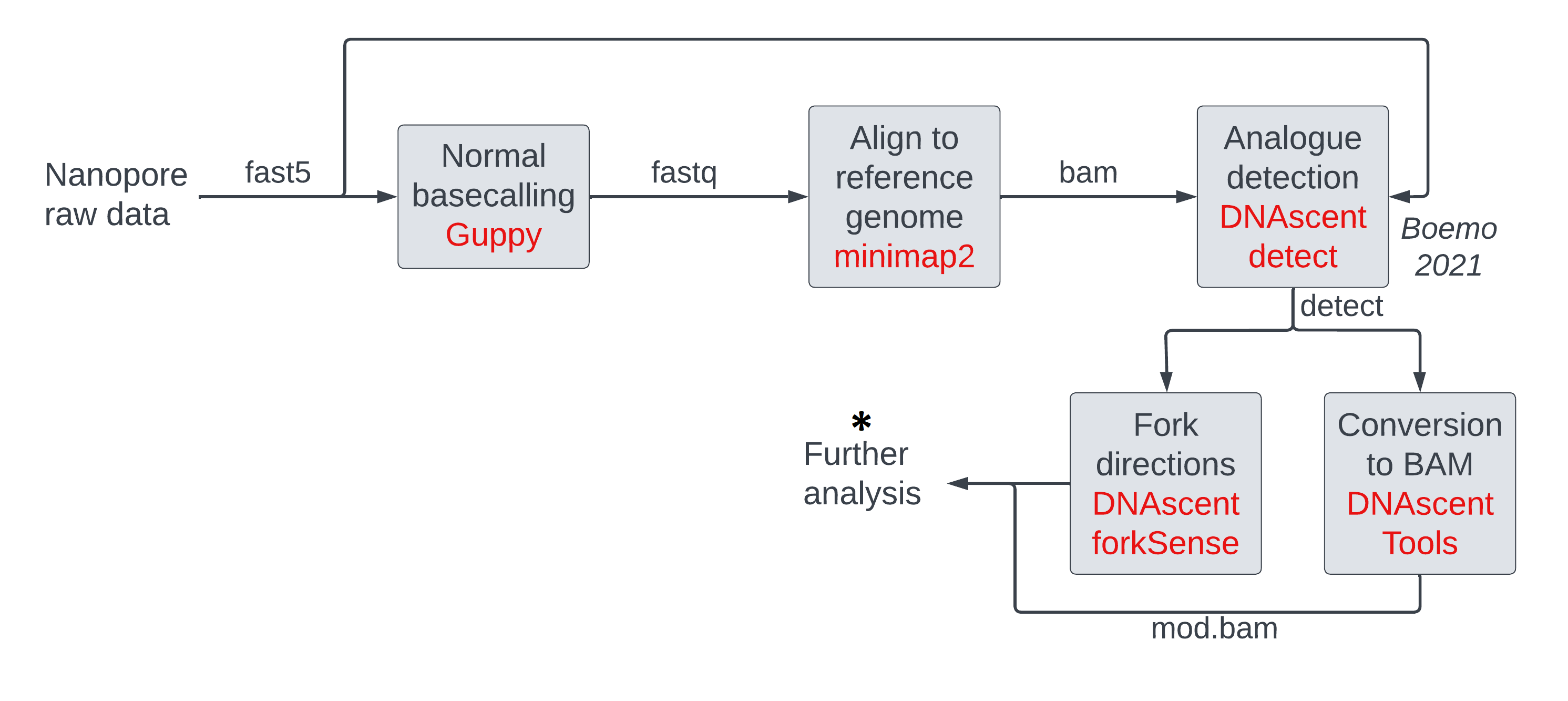
In this session, we will visualize modification data in mod BAM files (see figure below) using (1) genome
browsers (left) where we can rapidly scan data visually across different reads and different
regions on the genome, and (2) custom scripts (right) which allow us to see modification
density versus coordinate one read at a time.
We will discuss another visualization tool
modbamtools which produces visualizations such as
these
in a session tomorrow.
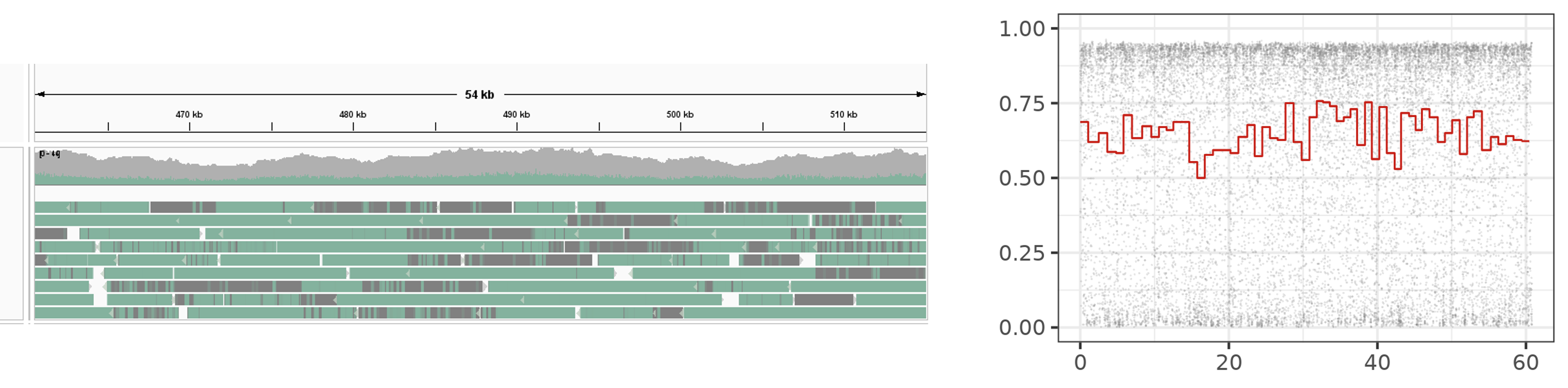
Either visualization has its strengths and weaknesses, which is why it is good to know how to do both. Genome browsers give you an overall idea and one can zoom in to regions on the genome and see data across multiple reads. But, beyond recognizing which regions are highly modified on a read (green) and which regions are not (grey), one cannot pick out any details of modification density such as gradients as there is no interpolation between the two colours to show any intermediary densities. Genome browsers cannot be used in a reference-unanchored workflow as they need a reference genome to produce visualizations. A related problem is that genome browsers ignore sections on reads corresponding to inserts i.e. sequences on the read which do not map to the genome.
On the right, we have plotted a read using a custom script, which shows raw modification data (grey) and windowed modification data (red). Here, we can see details per read but we cannot see multiple reads at the same time. We can visualize reads in a reference-dependent or reference-independent manner. We can also visualize one type of modification at a time if our file has multiple types of modifications on the same base. Genome browsers can visualize multiple modifications on the same base in some cases like 5mC and 5hmC.
We will explore the details of these visualizations and how to make them in this session. In the next session on manipulation of modification data, we will discuss how to do the equivalent of some of the analyses that goes on behind the scenes to make these visualizations (subsetting, thresholding, pileup, etc.) so that we can incorporate the commands in our own scripts.
Visualizing modification calls with IGV
Loading a mod BAM file
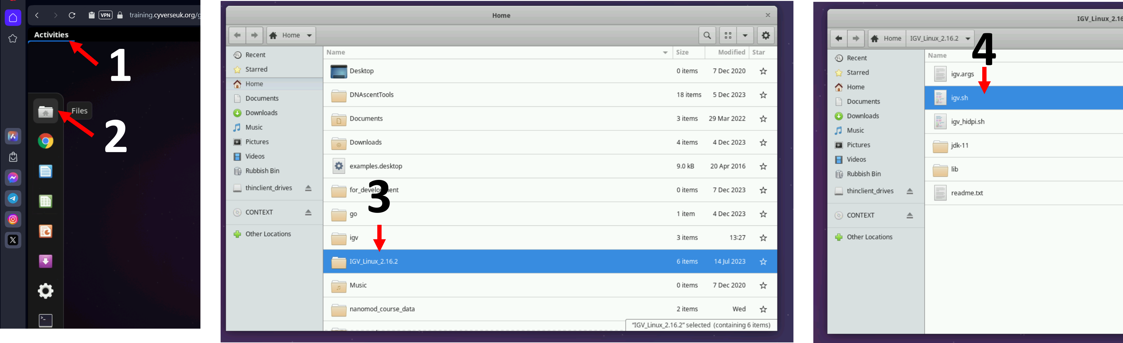
Let us open IGV on the virtual machines using the instructions from the figure below, like we did in the alignment session. If you are a self-study student, please open IGV on your computer.
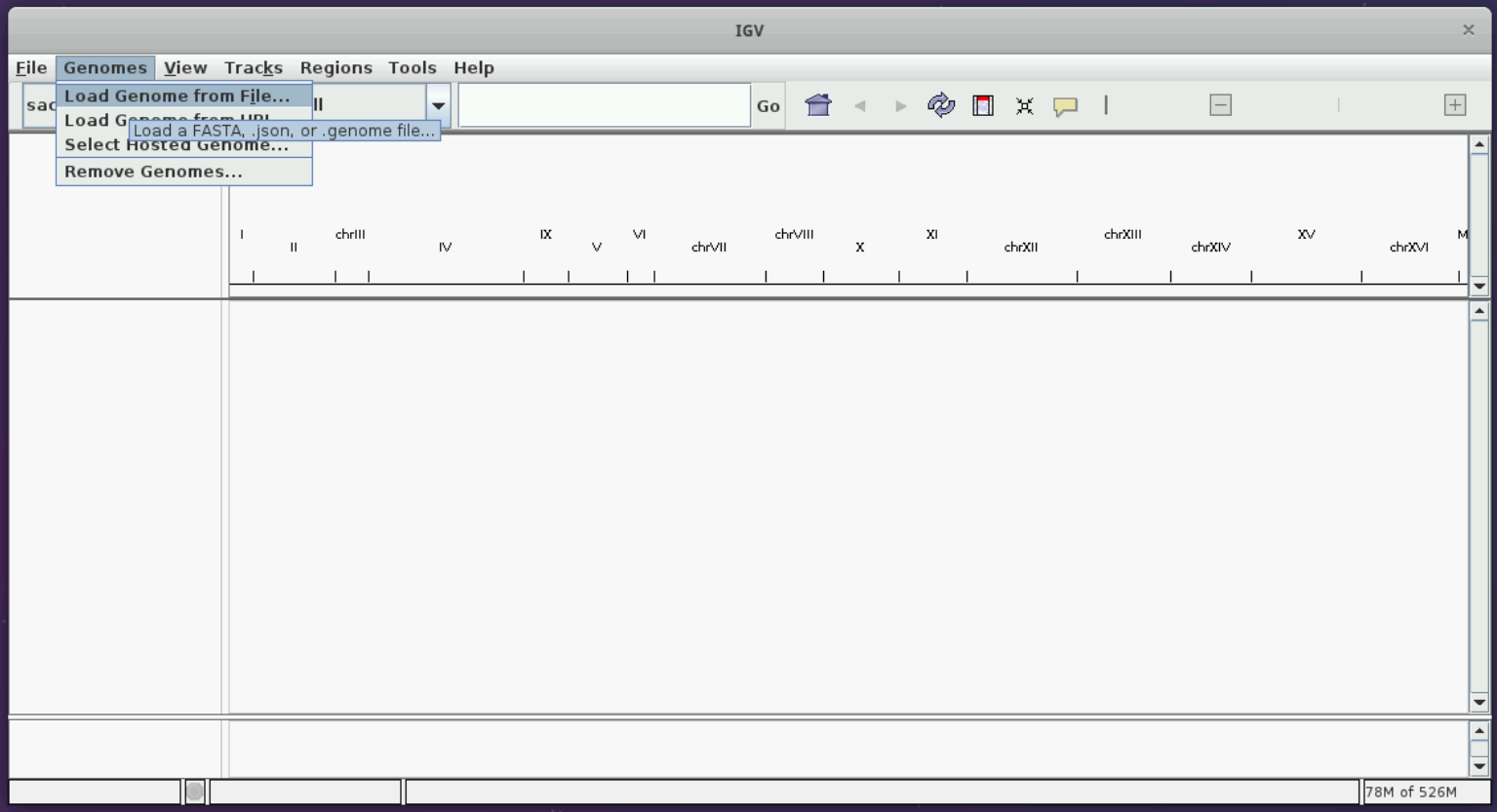
Let us load the sacCer3 genome and the mod BAM file produced from the yeast dataset in the modification calling session following the instructions in the figures below.
You should see two tracks immediately below the reference genome on top.
Colouring tracks by modification and exploring the visualization
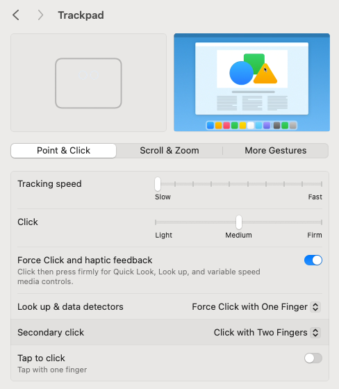
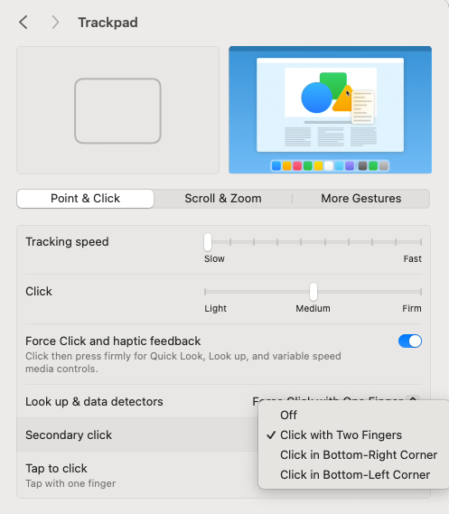
Now, we have to choose the option of ‘Color by modification’. Please follow the instructions in the figure below and please note that the colour you see in your IGV view may be different from the green shown here. You may have some issues if you are using a Mac trackpad; please see the helpful images here and here.
Now, you can zoom in to the genome. Select any region of size around 10 to 50 kb. You should see something similar to the figure below. Please note that the actual colours you see may be different.
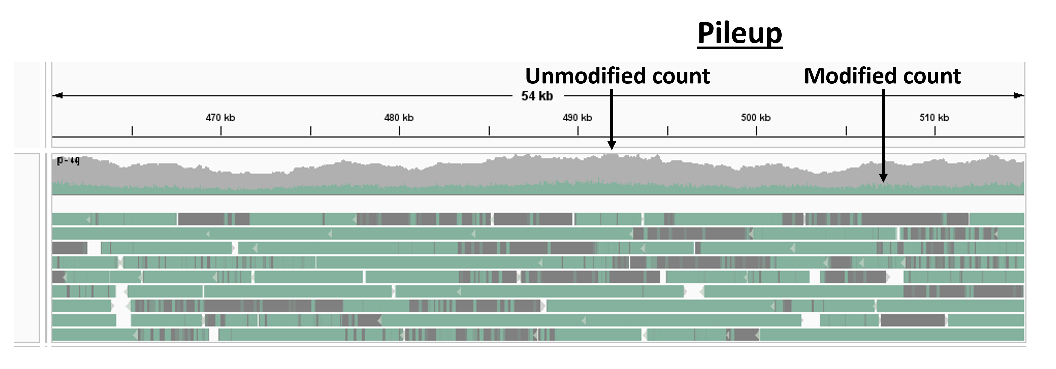
The gray and green tracks on top result from a pile-up analysis and show the modified and unmodified count versus genomic position (any averaging calculation that operates over all reads at every base on a reference genome is called a pile-up analysis).
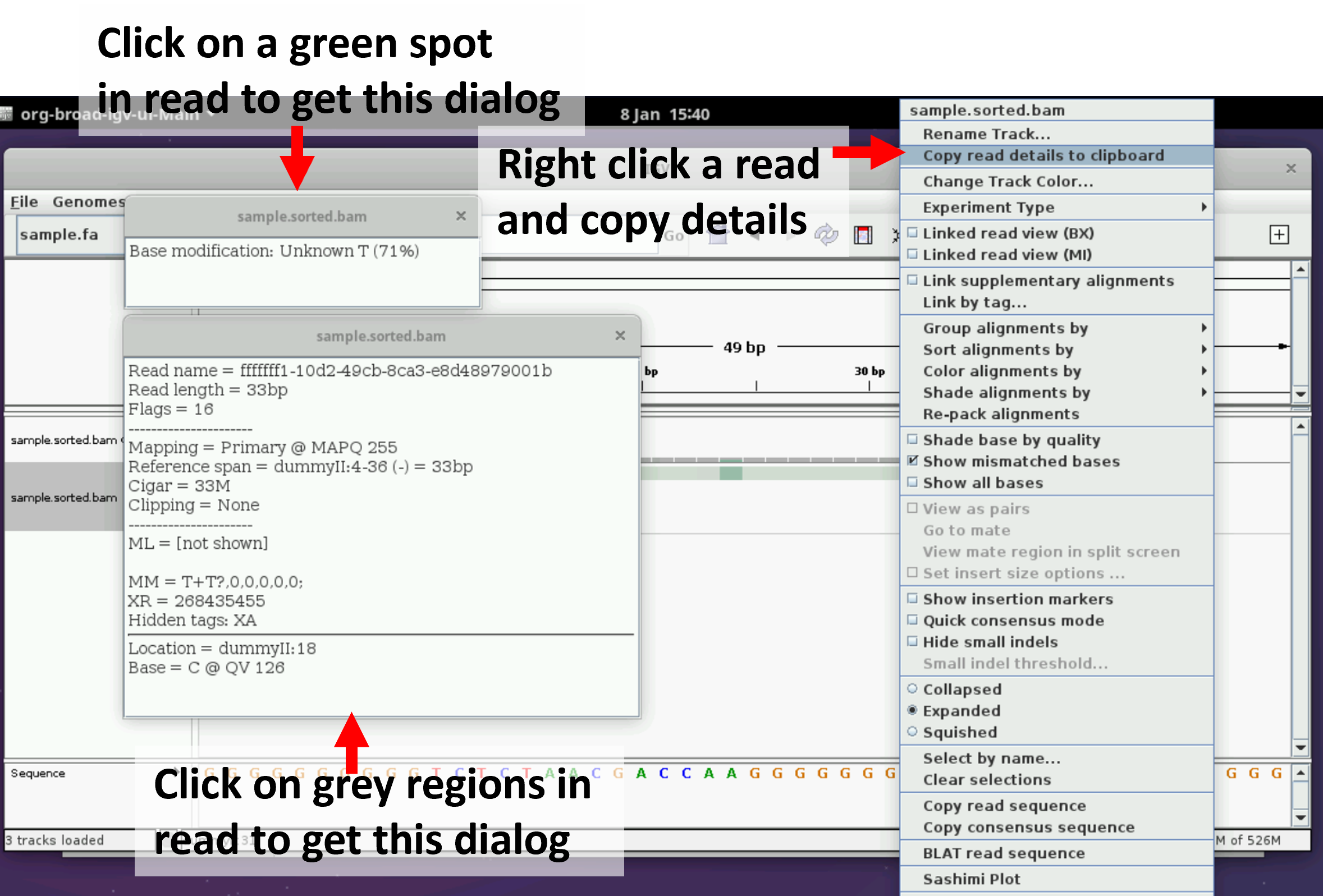
Try clicking on a read and see if you can get the following dialog boxes. They let you examine the modification probability of a single base on a read and extract read details such as read id.
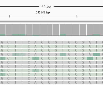
Try zooming in to a length scale of just a few bases. You should see individual bases marked as modified and unmodified.
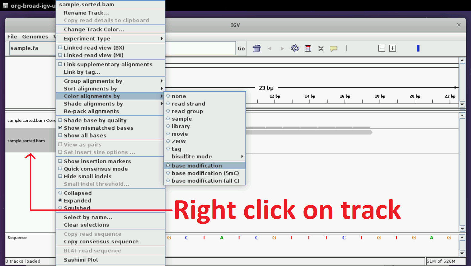
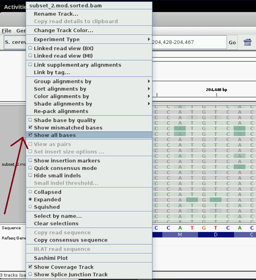
You may need to right click on the track and select “Show all bases” to see the bases overlaid on the green/grey colours in this view as shown in the figure below.
We can look at the reads for a few more minutes to get familiar with the visualization. Pick one or a few read ids of reads that look interesting to you and whose lengths are in the tens of kbs and record the details such as read id and location on the genome somewhere. When we visualize single molecules, you can visualize these molecules you’ve picked out.
Optional exercise
Exercise: Visualize reads around chrVI from a curated BAM file
We will visualize another mod BAM file in IGV in this exercise.
Visualizing modifications across single reads with custom script
We will now visualize a read of interest with our GUI program. First, we will get coordinates of all reads in our BAM file.
cd ~/nanomod_course_outputs/yeast
mod_bam=~/nanomod_course_outputs/yeast/dnascent.mod.sorted.bam
output_reads_bed=~/nanomod_course_outputs/yeast/reads_from_dnascent.bed
bedtools bamtobed -i $mod_bam > $output_reads_bed
# If you want to, you can inspect the first few lines of the output BED file
head -n 10 $output_reads_bed
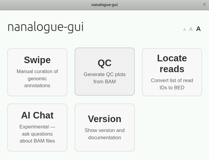
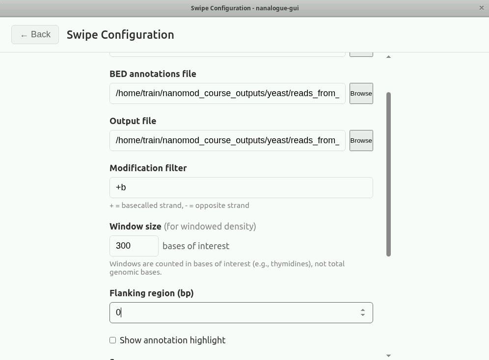
Now, run the command nanalogue-gui. Click on the Swipe button, then
load up the BAM file with the newly made BED file. You can choose
an appropriate name and location for the output bed file.
Uncheck ‘Show annotation highlight’ if checked and set ‘Flanking
Region’ to 0. Then press ‘Start Swiping’.
You should see two types of reads
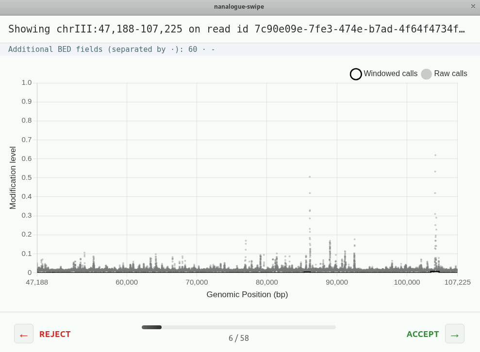
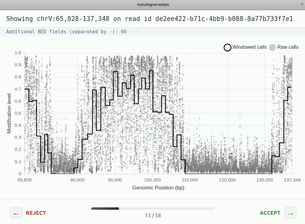
Compare the plot you see with the track of the same read in IGV. Can you pick out the same features?